Wine Quality Analysis
This project is done on a data set that can be found in the UCI Machine Learning Repository. It contains chemical information and quality score of both red and white Portuguese “Vinho Verde” wine. The goal is to model the quality score, a numeric from 1 to 10, of a wine based on its chemical properties. These properties include: alcohol percentage, density, which is mass of a wine, fixed acidity is the acids that give wine its flavor, volatile acidity can lead to a vinegar taste at high levels, and free sulfur dioxide prevents bacterial growth and oxidation.
Exploration
First we will look at the wine quality variable for both white and red wine.
par(mfrow=c(1,2))
counts = table(whitewine$quality)
barplot(counts, main = "White Wine")
counts2 = table(redwine$quality)
barplot(counts2, main = "Red Wine")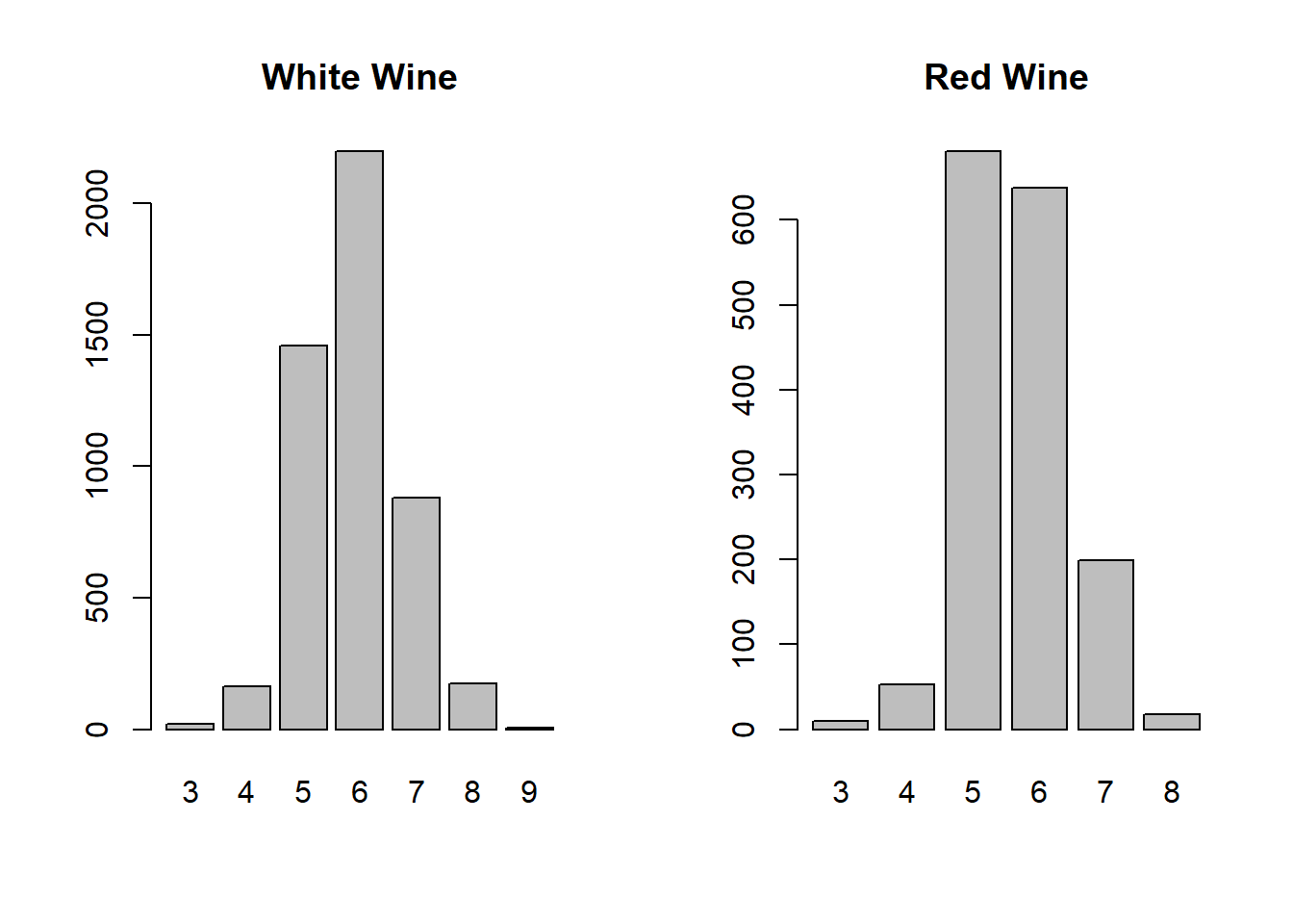
Here we can see that the distribution of quality scores is similar for both wines. Most wines are scored as a 5, 6, or 7. This is due to the fact that wine reviewers only give exceptional reviews to very good wines. We can already guess that any model will have a hard time predicting wines with very high or very low scores since the sample size is so small.
df = data.frame(correlations_w, correlations_r)
colnames(df) = c("white wine", "red wine")
df
## white wine red wine
## fixed.acidity -0.113662831 0.12405165
## volatile.acidity -0.194722969 -0.39055778
## citric.acid -0.009209091 0.22637251
## residual.sugar -0.097576829 0.01373164
## chlorides -0.209934411 -0.12890656
## free.sulfur.dioxide 0.008158067 -0.05065606
## total.sulfur.dioxide -0.174737218 -0.18510029
## density -0.307123313 -0.17491923
## pH 0.099427246 -0.05773139
## sulphates 0.053677877 0.25139708
## alcohol 0.435574715 0.47616632Before looking at the data I did some research on how wine quality is scored. Wine reviewers said that in general, wine with a high volatile acidity is bad. This is confirmed by these correlations between quality score and the other variables. Volatile acidity is negatively correlated, along with chlorides, total sulfur dioxide, and denisty. Interestingly, alcohol is positivly correlated with quality score. It is also the most correlated so it should be significant in modeling.
More Exploration w/ tree
my.control <- rpart.control(cp=0, xval=10)
fit1<- rpart(quality~., data=whitewine2[-train_white,], method="anova", control=my.control)
#printcp(fit1)
tree11 <-prune(fit1,cp=.009)
plot(tree11,uniform=T, margin=0.2)
text(tree11,use.n=T)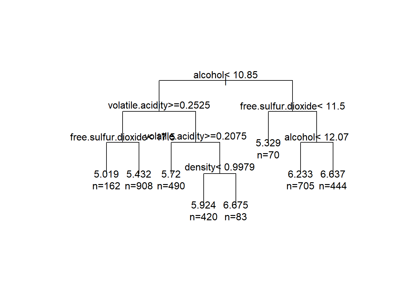
Here I made a single tree on my training data to see what the splits would look like. As expected, alcohol is an important split, being first. The rest of the splits are also the highly correlated variables.
Random Forest Regression
rf_w  = randomForest(quality~.,data=whitewine2[-train_white,], ntree=100, norm.votes=F)
print(rf_w)
##
## Call:
## randomForest(formula = quality ~ ., data = whitewine2[-train_white, ], ntree = 100, norm.votes = F)
## Type of random forest: regression
## Number of trees: 100
## No. of variables tried at each split: 3
##
## Mean of squared residuals: 0.3823454
## % Var explained: 50.17Here is a random forest on the white wine data. A regression forest was chosen since the response is numeric from 1-10. The % of variacne explained doesn’t seem great, so we will look at the testing data.
whitewine2$quality = factor(whitewine2$quality)
pred_w = round(predict(rf_w, whitewine2[train_white,]))

df1 = data.frame(pred_w,whitewine2[train_white,]$quality)
table(data.frame(pred_w,whitewine2[train_white,]$quality))
## whitewine2.train_white....quality
## pred_w 3 4 5 6 7 8 9
## 4 0 1 0 0 0 0 0
## 5 6 38 312 86 2 0 0
## 6 3 12 185 559 139 20 0
## 7 0 1 5 51 152 36 2
## 8 0 0 0 0 0 6 0The model is good at predicted average quality wines but not great at the more extreme qualities.
df1$acc = rep(0,1616)
df1$acc = as.numeric(df1$pred_w == df1$whitewine2.train_white....quality)
mean(df1$acc)
## [1] 0.6373762The testing accuracy ok at 67%
varImpPlot(rf_w)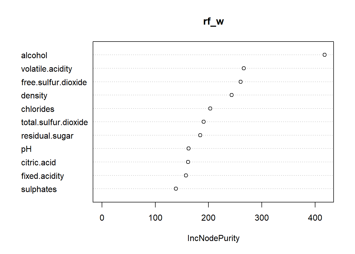
The variable important plot confirms our expectation of what variables were important for modeling.
3 levels
It is clear a regression random forest is not a fantastic way to predict wine quality. Predicting a specific score is difficult because of low sample size, so now we will try to predict a wine based on if it is good, average, or bad. A wine will be good if it is 7 or greater, average if it is a 5 or 6, and bad otherwise.
rf_w_gba  = randomForest(gba~.-quality,data=whitewine[-train_white,], ntree=100, norm.votes=F)
print(rf_w_gba)
##
## Call:
## randomForest(formula = gba ~ . - quality, data = whitewine[-train_white, ], ntree = 100, norm.votes = F)
## Type of random forest: classification
## Number of trees: 100
## No. of variables tried at each split: 3
##
## OOB estimate of error rate: 16.3%
## Confusion matrix:
## average bad good class.error
## average 2335 7 115 0.04965405
## bad 103 16 3 0.86885246
## good 307 0 396 0.43669986Here we can see a much smaller oob error rate. Part of the reason our error is so small is because the majority of wines are actually a 5 or 6, and the model predicts 5 or 6 the most.
pred_w = predict(rf_w_gba, whitewine[train_white,])
table(pred_w,whitewine[train_white,]$gba)
##
## pred_w average bad good
## average 1144 50 156
## bad 4 9 0
## good 50 2 201df2 = data.frame(pred_w,whitewine[train_white,]$gba)
df2$acc = as.numeric(df2$pred_w == df2$whitewine.train_white....gba)
mean(df2$acc)## [1] 0.8378713Our testing accuracy is much better, at ~84%.
Redwine
Lets see if red wine is much different than white in results. We will use a regression forest again here.
rf_r  = randomForest(quality~.,data=redwine[-train_red,], ntree=100, norm.votes=F)
print(rf_r)
##
## Call:
## randomForest(formula = quality ~ ., data = redwine[-train_red, ], ntree = 100, norm.votes = F)
## Type of random forest: regression
## Number of trees: 100
## No. of variables tried at each split: 3
##
## Mean of squared residuals: 0.3948705
## % Var explained: 39.57The model seems worse for the red wines, with even less variance explained.
redwine$quality = factor(redwine$quality)
pred_r = round(predict(rf_r, redwine[train_red,]))

df1 = data.frame(pred_r,redwine[train_red,]$quality)
table(data.frame(pred_r,redwine[train_red,]$quality))
## redwine.train_red....quality
## pred_r 3 4 5 6 7 8
## 5 5 28 330 101 7 0
## 6 3 7 122 304 92 6
## 7 0 0 1 19 38 3df1$acc = rep(0,1066)
df1$acc = as.numeric(df1$pred_r == df1$redwine.train_red....quality)
mean(df1$acc)## [1] 0.630394We can see the same trends here as with the white wine model, however the test accuracy is a little worse.
varImpPlot(rf_r)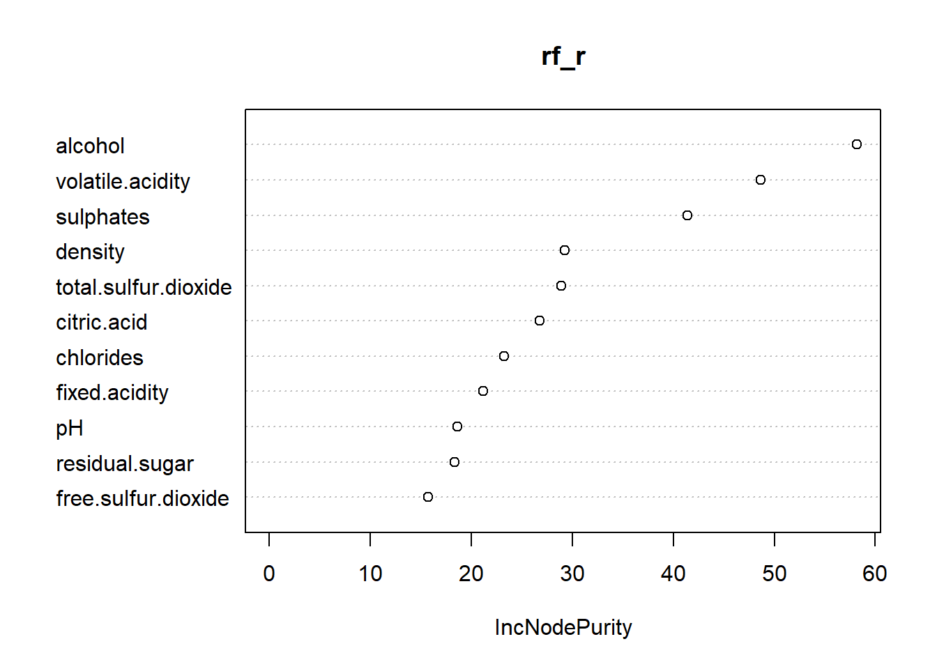
Here we can see that the important variables are similar, except for red wine sulphates is important.