Fake News Project
Our goal for this project was to look at how different political parties viewed fakes news. Our data set was from the PEW Research center and it contained question such as “How well do you think you can determine a fake news story”. These type of questions are the PEW questions which are:
PEW1: How often do you come across news stories about politics that you think are not totally accurate?
PEW2: And how often do you come across news stories about politics that you think completely made up?
PEW3: Have you shared a news story you later found out was made up?
PEW4: Have you shared a news story you thought at the time was made up?
PEW5a: How much responsibility do members of the public have in trying to prevent made up stories from gaining public attention? PEW5b: How much responsibility do government and elected officials have in trying to prevent made up stories from gaining public attention? PEW5c: How much responsibility do social media websites have in trying to prevent made up stories from gaining public attention? PEW6: How confident are you in your ability to recognize news that is made up?
PEW7: How much do you think these kind of stories leave Americans confused about the basic facts of current events?
First we looked at how the political variables were distributed.
Political Affiliations of Population
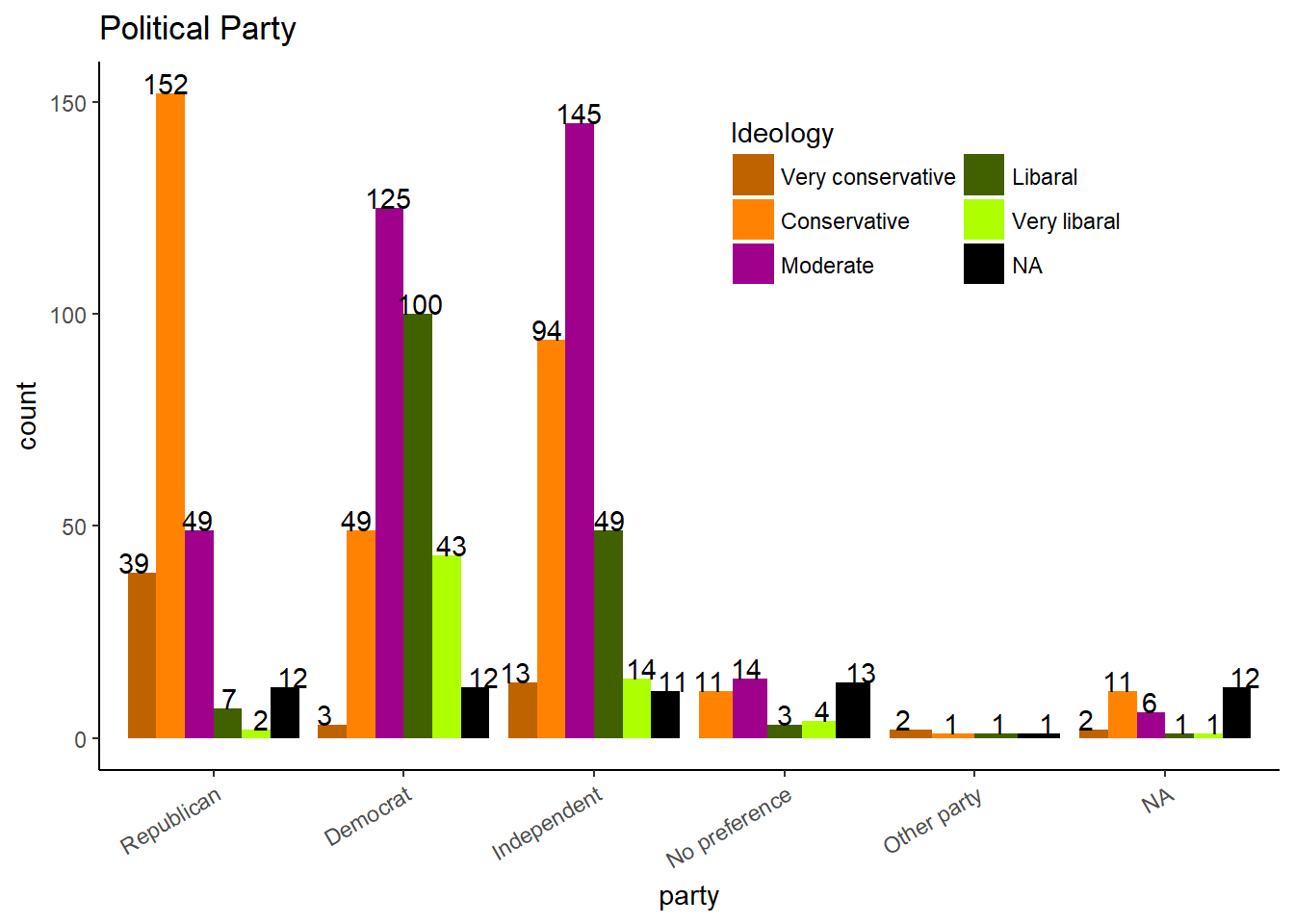
Here we looked at political party and political ideology. A few of the responses were odd, with a couple very liberal republicans or very conservative democrats.
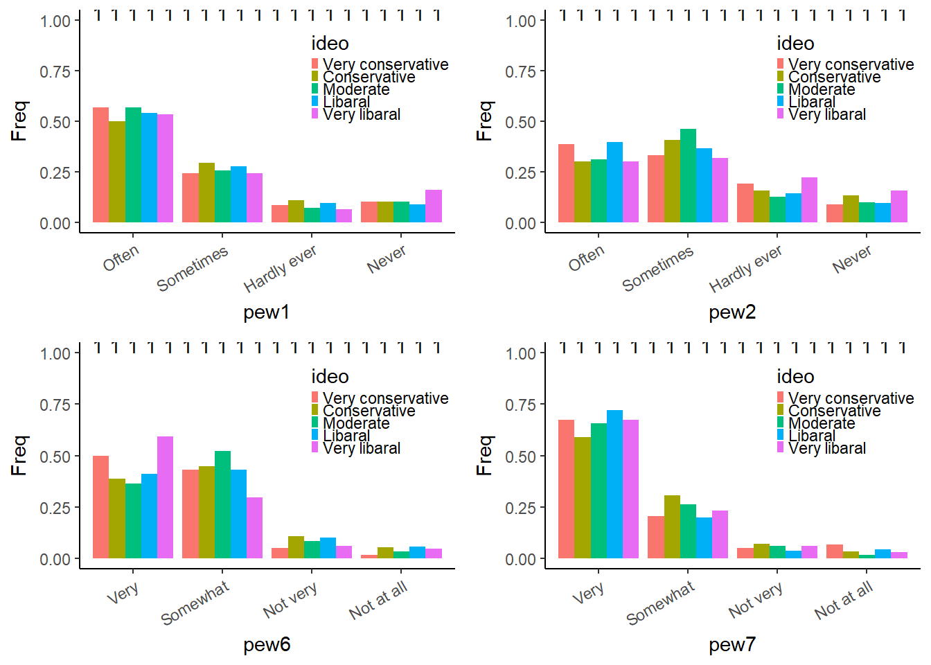
Pew questions vs Ideology
## TableGrob (2 x 2) "arrange": 4 grobs
##   z     cells    name           grob
## 1 1 (1-1,1-1) arrange gtable[layout]
## 2 2 (1-1,2-2) arrange gtable[layout]
## 3 3 (2-2,1-1) arrange gtable[layout]
## 4 4 (2-2,2-2) arrange gtable[layout]
Then we looked at how the PEW questions distributed across ideology. We can see that answers for the PEW questions do sometimes differ among ideologies. Specifically people who are very liberal or very conservative have stronger beliefs about PEW6. Now we will try to create a model.
##
## Call:
## glm(formula = ideo ~ . - ideo, family = "binomial", data = pew2,
##     subset = train)
##
## Deviance Residuals:
##     Min       1Q   Median       3Q      Max
## -2.7510   0.2817   0.4283   0.5775   1.1739
##
## Coefficients:
##                              Estimate Std. Error z value Pr(>|z|)
## (Intercept)                  1.008013   1.071018   0.941   0.3466
## pew1Sometimes               -0.047090   0.364739  -0.129   0.8973
## pew1Hardly ever              0.886616   0.647197   1.370   0.1707
## pew1Never                   -0.022220   0.678448  -0.033   0.9739
## pew2Sometimes                0.032393   0.358796   0.090   0.9281
## pew2Hardly ever             -0.999715   0.437905  -2.283   0.0224 *
## pew2Never                    0.036962   0.677376   0.055   0.9565
## pew3No                       0.404138   0.401597   1.006   0.3143
## pew4No                      -0.420114   0.477448  -0.880   0.3789
## pew5aA fair amount           0.204185   0.323809   0.631   0.5283
## pew5aNot much                0.125621   0.467866   0.268   0.7883
## pew5aNone at all             0.771980   0.607229   1.271   0.2036
## pew5bA fair amount           0.408030   0.389274   1.048   0.2946
## pew5bNot much               -0.130600   0.397221  -0.329   0.7423
## pew5bNone at all            -0.797607   0.462056  -1.726   0.0843 .
## pew5cA fair amount           0.382967   0.340452   1.125   0.2606
## pew5cNot much                1.145835   0.594189   1.928   0.0538 .
## pew5cNone at all            -0.027009   0.460387  -0.059   0.9532
## pew6Somewhat                 0.465761   0.297634   1.565   0.1176
## pew6Not very                 1.278106   0.704661   1.814   0.0697 .
## pew6Not at all               1.068713   0.893933   1.196   0.2319
## pew7Somewhat                 0.543345   0.352043   1.543   0.1227
## pew7Not very                 0.922069   0.813524   1.133   0.2570
## pew7Not at all              -0.513668   0.787039  -0.653   0.5140
## sexFemale                    0.185620   0.278787   0.666   0.5055
## age                          0.002175   0.007534   0.289   0.7728
## educ2High school incomplete -1.082103   1.022023  -1.059   0.2897
## educ2High school graduate    0.083834   0.907505   0.092   0.9264
## educ2Some college           -0.259900   0.927357  -0.280   0.7793
## educ2Associate degree        0.884577   1.013526   0.873   0.3828
## educ2Bachelor degree         0.051435   0.909573   0.057   0.9549
## educ2Some postgraduate      -0.712975   1.212864  -0.588   0.5566
## educ2Postgraduate            0.185515   0.925536   0.200   0.8411
## ---
## Signif. codes:  0 '***' 0.001 '**' 0.01 '*' 0.05 '.' 0.1 ' ' 1
##
## (Dispersion parameter for binomial family taken to be 1)
##
##     Null deviance: 417.19  on 528  degrees of freedom
## Residual deviance: 376.60  on 496  degrees of freedom
##   (139 observations deleted due to missingness)
## AIC: 442.6
##
## Number of Fisher Scoring iterations: 5
After selecting all of the PEW questions and a couple of extra variables, we created a logistic model. The dependent variable here is political ideology. We changed the variable from 5 levels to just 2, extreme and moderate. Extreme included people who were very liberal and very conservative. Moderate was everything else. We also seperated the data into a training dataset to build the model and a testing set for later.
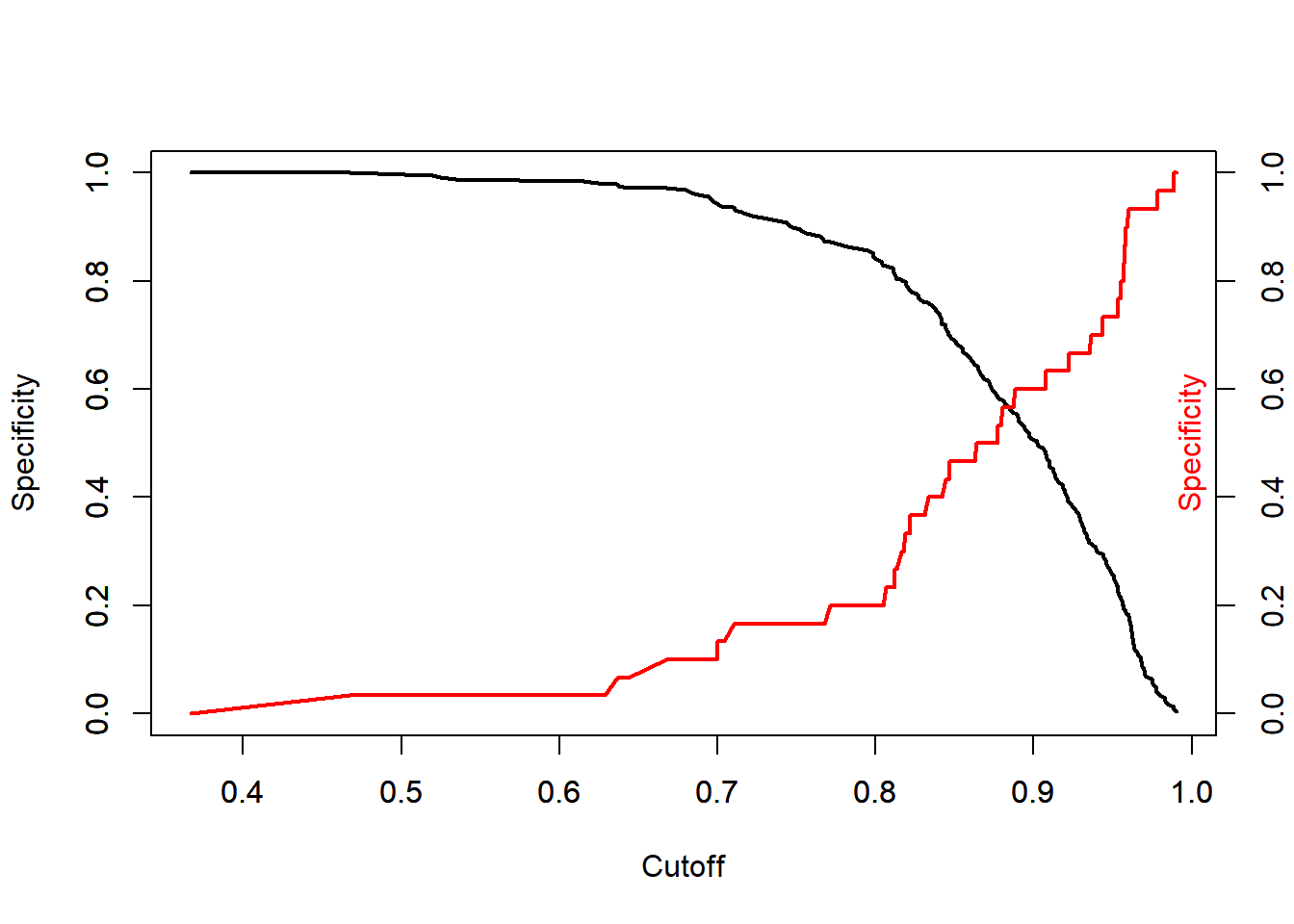
With a glm we need to find a cutoff point for what group a probability goes into, either moderate of extreme. We do this by looking at a graph of possible sensitivities and specificities. We choose the x value where they intersect. This maximizes sensitivity and specificity. We wont be biased towards positives or negatives. Since this is all an estimation and its impossible to be exact, we’ll just go with .89. So, in this model a true positive for extreme will be less than .89 and a true negative for moderate will be greater than .89.
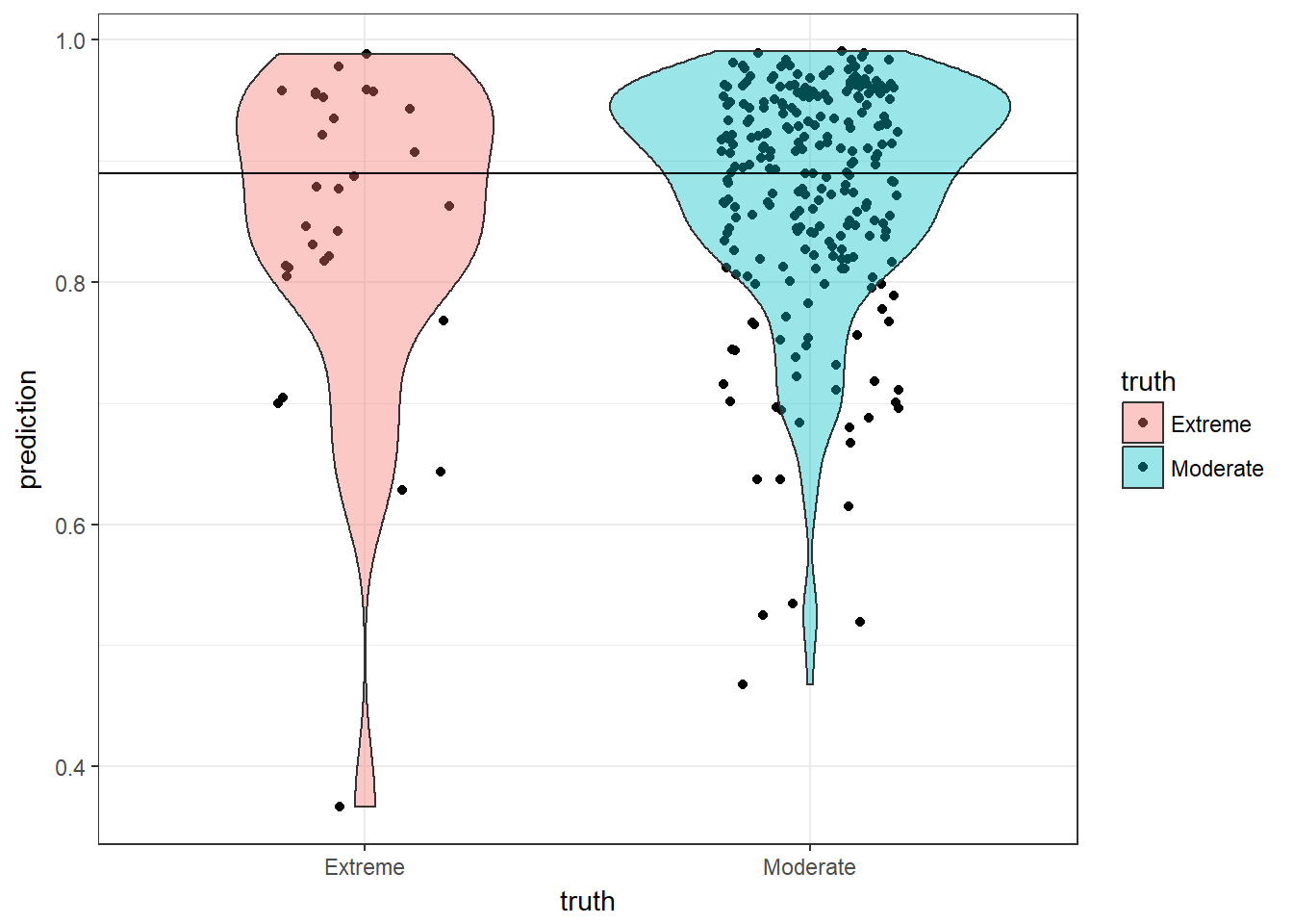
This plot shows that we chose a good cutoff. For the moderates, most of them are above the line. If the line was any higher we would predict too many moderates falsely.
## Confusion Matrix and Statistics
##
##           Reference
## Prediction Extreme Moderate
##   Extreme       18      113
##   Moderate      12      137
##
##                Accuracy : 0.5536
##                  95% CI : (0.4933, 0.6127)
##     No Information Rate : 0.8929
##     P-Value [Acc > NIR] : 1
##
##                   Kappa : 0.0596
##  Mcnemar's Test P-Value : <2e-16
##
##             Sensitivity : 0.60000
##             Specificity : 0.54800
##          Pos Pred Value : 0.13740
##          Neg Pred Value : 0.91946
##              Prevalence : 0.10714
##          Detection Rate : 0.06429
##    Detection Prevalence : 0.46786
##       Balanced Accuracy : 0.57400
##
##        'Positive' Class : Extreme
##
Our model had a 55% accuracy rate. The specificity (true negative rate) is better at 60% and the sensitivity (true positive rate) is average at 54%. This could be because of the low sample size of extreme ideologies. Next we made a model with political party being the dependent variable.
## [1] "Republican"    "Democrat"      "Independent"   "No preference"
## [5] "Other party"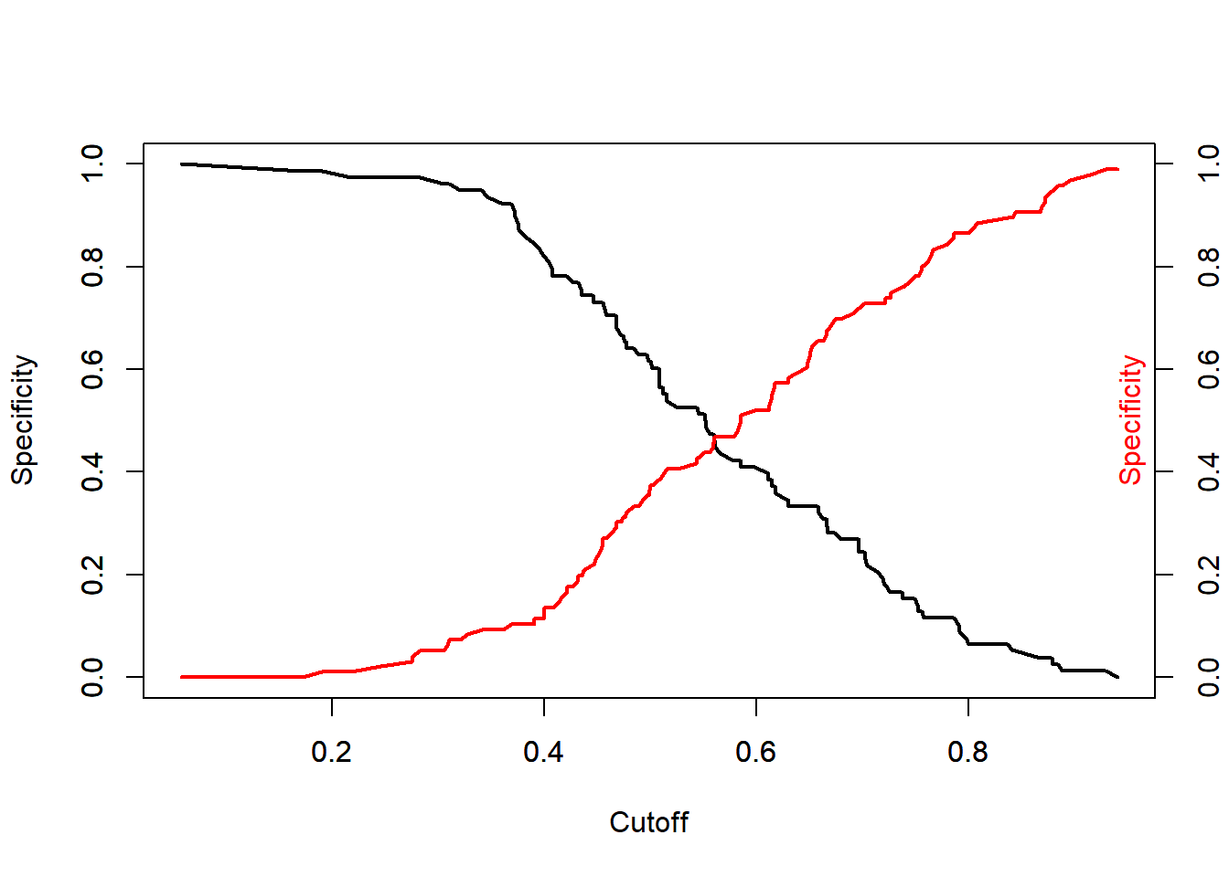
This time our cutoff will be .52.
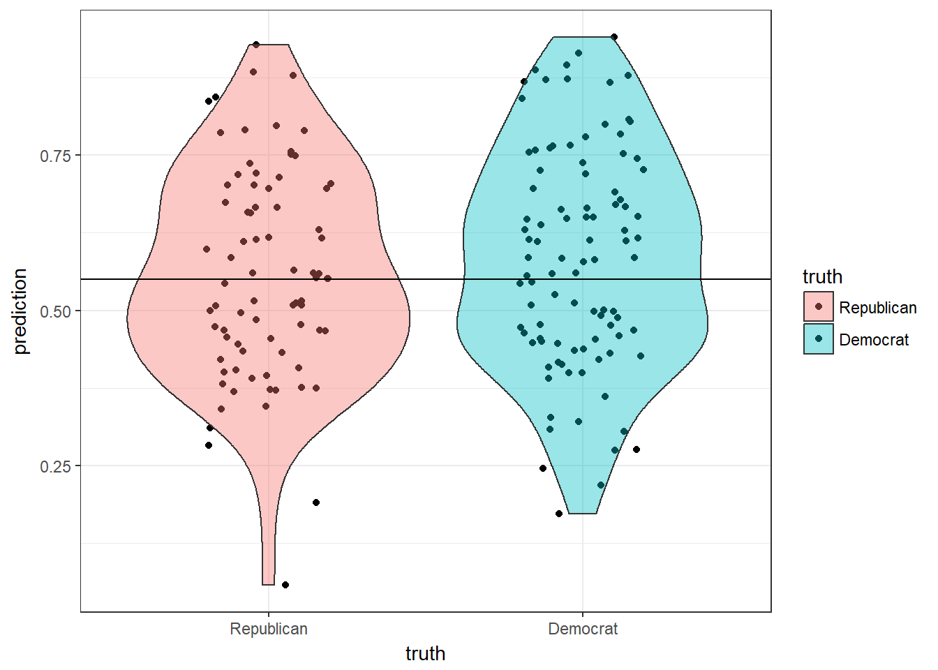
This time republican is a positive and democrat is a negative. Again, we should have a higher specificity than sensitivity.
## Confusion Matrix and Statistics
##
##             Reference
## Prediction   Republican Democrat
##   Republican         38       42
##   Democrat           40       54
##
##                Accuracy : 0.5287
##                  95% CI : (0.4518, 0.6047)
##     No Information Rate : 0.5517
##     P-Value [Acc > NIR] : 0.7540
##
##                   Kappa : 0.0496
##  Mcnemar's Test P-Value : 0.9121
##
##             Sensitivity : 0.4872
##             Specificity : 0.5625
##          Pos Pred Value : 0.4750
##          Neg Pred Value : 0.5745
##              Prevalence : 0.4483
##          Detection Rate : 0.2184
##    Detection Prevalence : 0.4598
##       Balanced Accuracy : 0.5248
##
##        'Positive' Class : Republican
##
This model is also not very accurate. It has a higher specificity than the previous model, but thats the only improvement.
Overall these models showed that accurate predictions should be possible with better data. I think with a higher sample size and more specific questions political ideology can be predicted with fake news opinions.