Confirmatory Factor Analysis
For this project I was given a data set where the researchers had an idea of how the variables would relate. These were nine factors about emotional health and our goal was to see if the variables would be grouped into these nine factors through confirmatory factor analysis. Only a couple were close and the rest were far from it.
Since our goal was to see how the variables related, I first looked at how R would group the variables.
Data Exploration for factor analysis
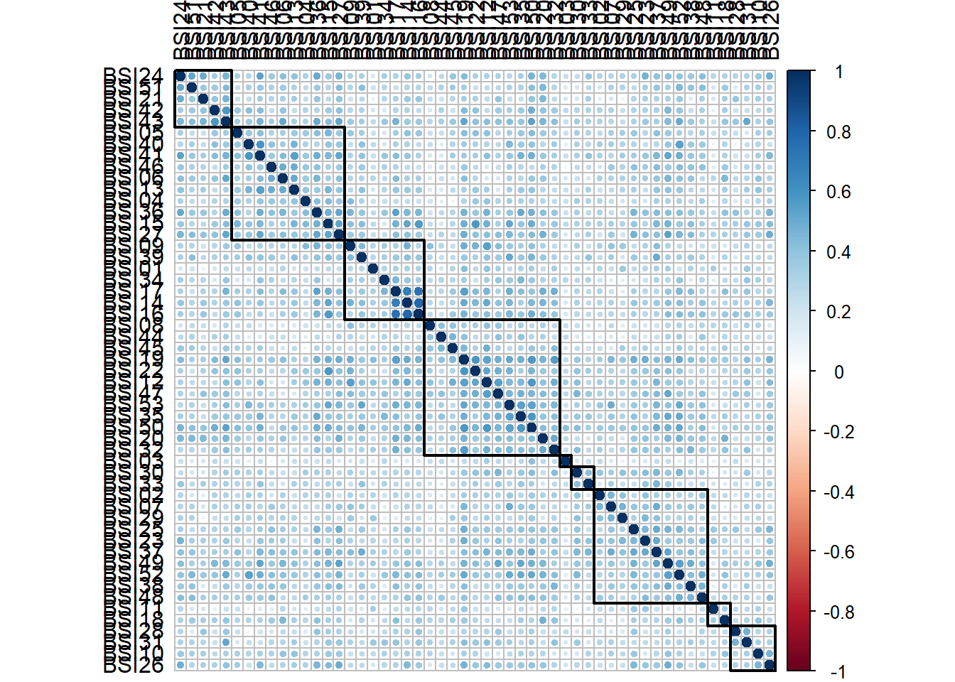
This first plot is called a corrplot. Corrplots try to group variables that are highly correlated into however many groups we want. This corrplot has some very small groupings of variables when it is forced to do nine. This may leave us with some lackluster factors that do not fit what is predicted.
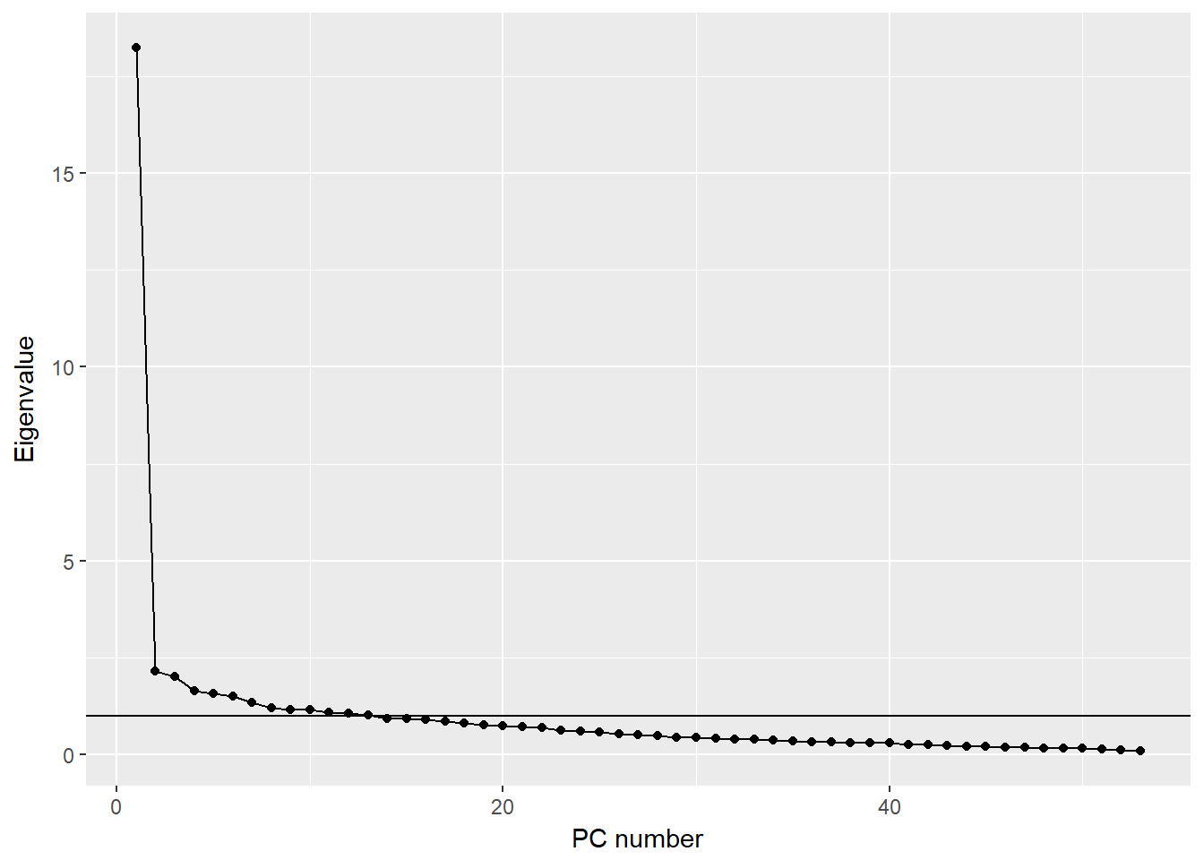
This second plot is a scree plot. It looks at the eigenvalues to determine how many factors we should have. The scree plot tells us that we could take 2 factors if we followed the elbow rule or about 12 factors if we choose to go for an eigenvalue less than 1. We will still try 9 since that is what is expected. Now we will look at the factor loadings, given that there should be 9 factors.
Factors and their loadings
##
## Loadings:
##       RC3    RC5    RC2    RC8    RC1    RC4    RC7    RC6    RC9
## BSI01  0.451
## BSI02  0.550
## BSI03
## BSI04                       0.479
## BSI05                       0.450
## BSI06                0.614
## BSI07  0.643
## BSI08                                            0.667
## BSI09                       0.656
## BSI10                0.490
## BSI11                                                          0.624
## BSI12                       0.547
## BSI13                0.679
## BSI14         0.729
## BSI15         0.470         0.493
## BSI16         0.797
## BSI17         0.797
## BSI18
## BSI19         0.448
## BSI20
## BSI21                                     0.635
## BSI22                       0.565
## BSI23  0.560                              0.537
## BSI24                                     0.685
## BSI25  0.406
## BSI26
## BSI27                              0.480
## BSI28                                                   0.698
## BSI29  0.685
## BSI30  0.586
## BSI31                                                   0.555
## BSI32         0.460
## BSI33                                     0.429
## BSI34                                                   0.475
## BSI35
## BSI36
## BSI37  0.544
## BSI38  0.490
## BSI39
## BSI40                0.572
## BSI41                0.522
## BSI42                              0.658
## BSI43                              0.436
## BSI44                                            0.654
## BSI45                                            0.567
## BSI46                0.604
## BSI47
## BSI48
## BSI49                              0.528
## BSI50
## BSI51                                     0.500
## BSI52
## BSI53
##
##                  RC3   RC5   RC2   RC8   RC1   RC4   RC7   RC6   RC9
## SS loadings    4.809 4.653 4.251 3.669 3.628 3.200 3.066 2.276 1.507
## Proportion Var 0.091 0.088 0.080 0.069 0.068 0.060 0.058 0.043 0.028
## Cumulative Var 0.091 0.179 0.259 0.328 0.396 0.457 0.515 0.558 0.586
Factor 1 (RC1): BSI03,04,05,09,12,15,22,50,53. BSI Obsessive compulsive subscale
Factor 2 (RC4): BSI07,25,35,37,38,46,47,48,49,52,53. BSI Anxiety subscale
Factor 3 (RC9): BSI20,21,24,41,42,43,51. BSI Interpersonal sensitivity subscale
Factor 4 (RC5): BSI14,15,16,17,32. BSI Depression subscale
Factor 5 (RC2): BSI04,06,10,13,40,41,46. BSI Hostility subscale
Factor 6 (RC3): BSI01,02,07,23,29,30. Somatization subscale
These factors are not associating as expected. After factor 6, the rest of the factors do not contain nearly enough of the expected variables to be considered close to the expected. Now we will create a model to predict the overprotection subscale in the data.
Data exploration for model building
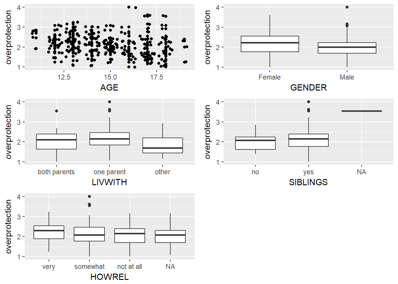
From some bivariate graphs of demographic variables vs overprotection we can see that there may be a relationship between age and overprotection. Females may have a higher overprotection than males. Living situation may be something that effects overprotection. Both having siblings and religiousness do not seem very significant.
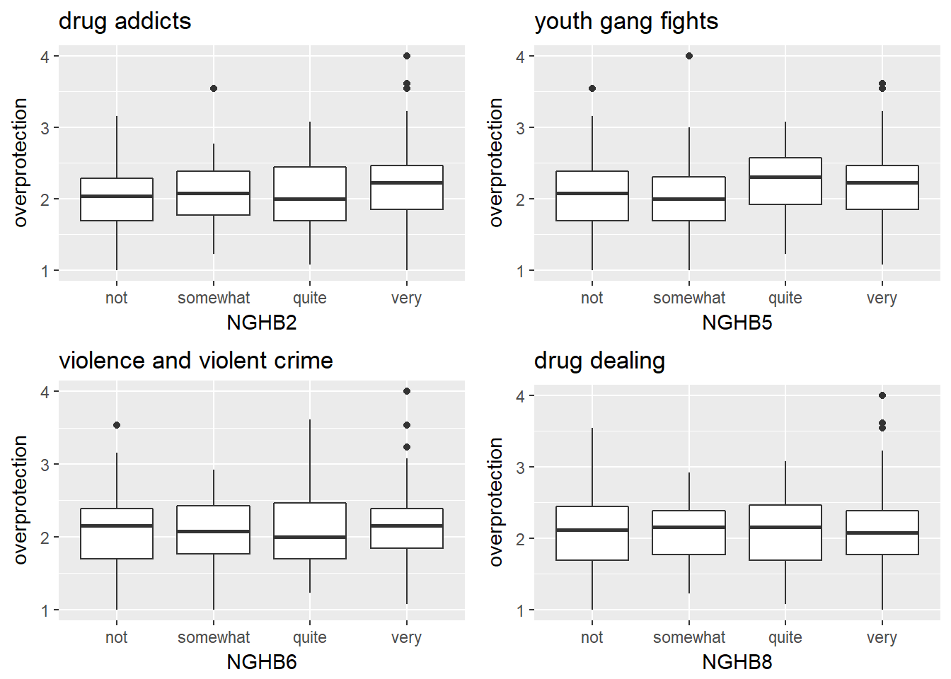
For the neighborhood variables it looks like drug addicts in the neighborhood and youth gang fights may effect overprotection. Violence and drug dealing to not seem significant.
Model building
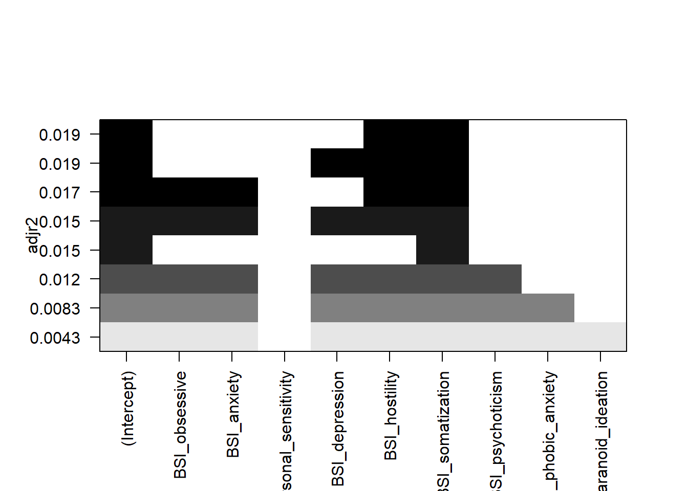
For this first model I will just use the BSI variables that maximize R^2 and some demographic variables.
First we will see what automatic variable selection thinks.
##                   (Intercept)                 BSI_obsessive
##                          TRUE                         FALSE
##                   BSI_anxiety BSI_interpersonal_sensitivity
##                         FALSE                         FALSE
##                BSI_depression                 BSI_hostility
##                          TRUE                          TRUE
##              BSI_somatization              BSI_psychoticism
##                          TRUE                         FALSE
##            BSI_phobic_anxiety         BSI_paranoid_ideation
##                         FALSE                         FALSE
BSI_depression, BSI_hostility, and BSI_somatization seem to be significant variables.
| Estimate | Std. Error | t value | |
|---|---|---|---|
| (Intercept) | 2.791 | 0.2522 | 11.07 |
| AGE | -0.04386 | 0.01659 | -2.644 |
| LIVWITHone parent | 0.1405 | 0.08397 | 1.673 |
| LIVWITHother | -0.1642 | 0.133 | -1.234 |
| GENDERMale | -0.2211 | 0.06443 | -3.432 |
| BSI_interpersonal_sensitivity | 0.01263 | 0.03198 | 0.3949 |
| BSI_hostility | 0.05103 | 0.03279 | 1.556 |
| BSI_paranoid_ideation | -0.0009373 | 0.03187 | -0.02941 |
| Pr(>|t|) | |
|---|---|
| (Intercept) | 2.981e-23 |
| AGE | 0.00874 |
| LIVWITHone parent | 0.09567 |
| LIVWITHother | 0.2185 |
| GENDERMale | 0.0007065 |
| BSI_interpersonal_sensitivity | 0.6933 |
| BSI_hostility | 0.1209 |
| BSI_paranoid_ideation | 0.9766 |
| Observations | Residual Std. Error | \(R^2\) | Adjusted \(R^2\) |
|---|---|---|---|
| 247 | 0.4927 | 0.1371 | 0.1119 |
## [1] 361.1086This model is not great, with at adjusted R^2 of .1119. Lets see if we can make it better.
For the second model I will try forward selection starting with age and then add neighborhood and bsi variables.
Similarialy I made a second model.
| Estimate | Std. Error | t value | Pr(>|t|) | |
|---|---|---|---|---|
| (Intercept) | 2.798 | 0.2464 | 11.36 | 3.768e-24 |
| AGE | -0.05254 | 0.01669 | -3.148 | 0.001855 |
| BSI_hostility | 0.06349 | 0.03333 | 1.905 | 0.05796 |
| BSI_somatization | 0.04944 | 0.03413 | 1.448 | 0.1488 |
| NGHB2somewhat | 0.205 | 0.1258 | 1.629 | 0.1046 |
| NGHB2quite | 0.3332 | 0.1481 | 2.249 | 0.02542 |
| NGHB2very | 0.4447 | 0.1354 | 3.283 | 0.001182 |
| NGHB8somewhat | -0.06436 | 0.1245 | -0.5168 | 0.6058 |
| NGHB8quite | -0.2795 | 0.1486 | -1.881 | 0.06117 |
| NGHB8very | -0.2952 | 0.1335 | -2.211 | 0.02797 |
| Observations | Residual Std. Error | \(R^2\) | Adjusted \(R^2\) |
|---|---|---|---|
| 247 | 0.5027 | 0.109 | 0.07519 |
## [1] 373.0254This model is also not great, but maybe if we combine the models it will be better.
Model 1 has a adjusted R^2 of .111 and a AIC of 361.1. Model 2 has an adjusted R^2 of .075 and an AIC of 373.02. Model 1 is a better model. For the final model we will add the effective variables in model 2 to model 1.
| Estimate | Std. Error | t value | Pr(>|t|) | |
|---|---|---|---|---|
| (Intercept) | 2.627 | 0.2582 | 10.17 | 2.343e-20 |
| AGE | -0.04157 | 0.01713 | -2.427 | 0.01599 |
| LIVWITHone parent | 0.1448 | 0.08313 | 1.742 | 0.08274 |
| LIVWITHother | -0.196 | 0.1339 | -1.464 | 0.1446 |
| GENDERMale | -0.1869 | 0.06516 | -2.869 | 0.004498 |
| BSI_hostility | 0.05259 | 0.03255 | 1.616 | 0.1075 |
| BSI_paranoid_ideation | -0.01988 | 0.0322 | -0.6174 | 0.5376 |
| BSI_somatization | 0.03246 | 0.03353 | 0.9682 | 0.334 |
| NGHB2somewhat | 0.1937 | 0.1224 | 1.583 | 0.1147 |
| NGHB2quite | 0.2918 | 0.147 | 1.986 | 0.04824 |
| NGHB2very | 0.3978 | 0.1351 | 2.944 | 0.003573 |
| NGHB8somewhat | 0.0157 | 0.1225 | 0.1282 | 0.8981 |
| NGHB8quite | -0.2149 | 0.1451 | -1.481 | 0.1399 |
| NGHB8very | -0.2409 | 0.1318 | -1.828 | 0.0689 |
| Observations | Residual Std. Error | \(R^2\) | Adjusted \(R^2\) |
|---|---|---|---|
| 247 | 0.4864 | 0.18 | 0.1343 |
## [1] 360.5092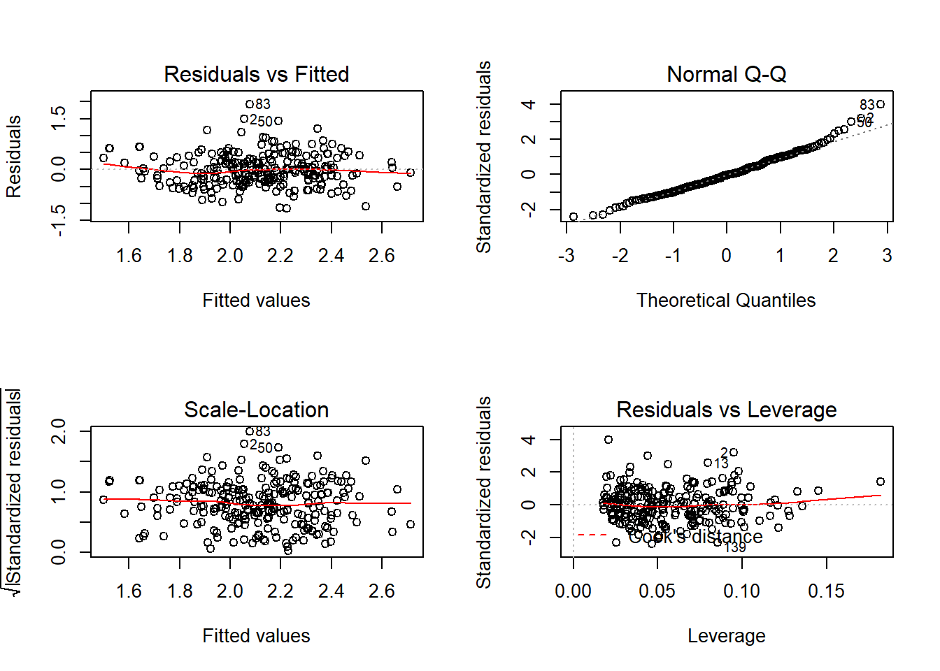
This model has an adjusted R^2 of .134 and an AIC of 360.509, making it the best model. The residuals of this model are mostly normal. For our coefficients we have -.04(age) which is a -.04 decrease in overprotection as age decreases. There is .144 increasing for living with one parent when compared to two parents and -.19 for other. There is -.1869 decrease in overprotection for males when compared to females. For BSI-hostility there is a .05 increase for each increase in the score. There is a -.01 decrease and a .032 increase for BSI_paranoid_ideation and BSI somatization respectively. For NGHB2, drug addicts in a neighborhood, we have .19 increase if it is somewhat a problem, .291 if it is quite a problem, and .397 if it is very much a problem. Finally for NGHB8, drug dealing, we have a .015 increase if it is somewhat a problem, -.214 decrease if it is quite a problem, and -.24 decrease if it is very much a problem.